Concentric 3rd and 4th order rainbows at Dresden-Langebrück, Aug 11th, 2020

17:27:54 CEST, Pentax K-5, smc Pentax-DA fisheye 10-17 mm at f = 10 mm, f/8, 1/1600 s at ISO 80, artifact-minimized processing by separate unsharp masking of color differences

Original image

Green minus blue color channel difference unsharp masked

Color differences unsharp masked

Taking photographs of tertiary and quaternary rainbows is difficult, as usually you won’t see what you are aiming at – theory predicts that the tertiary is just at the threshold of visibility [1], and for the quaternary the situation is even worse. I myself have been lucky only once before [2], (though having tried for almost a decade now), if one does not count experiments using artificial sprays [3]. This cannot be attributed to a lack of opportunities. Over the years, I experienced several promising situations, but afterwards no higher order rainbows could be extracted from the photographs by image processing. One problem is that cloud structures in the background mess up the unsharp mask filter. But maybe also my timing was just wrong and these rainbows did not appear when I expect them to do, because I misjudged the shower and illumination geometry.

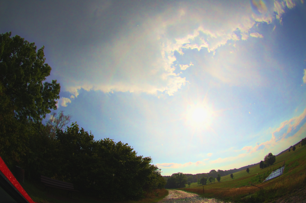
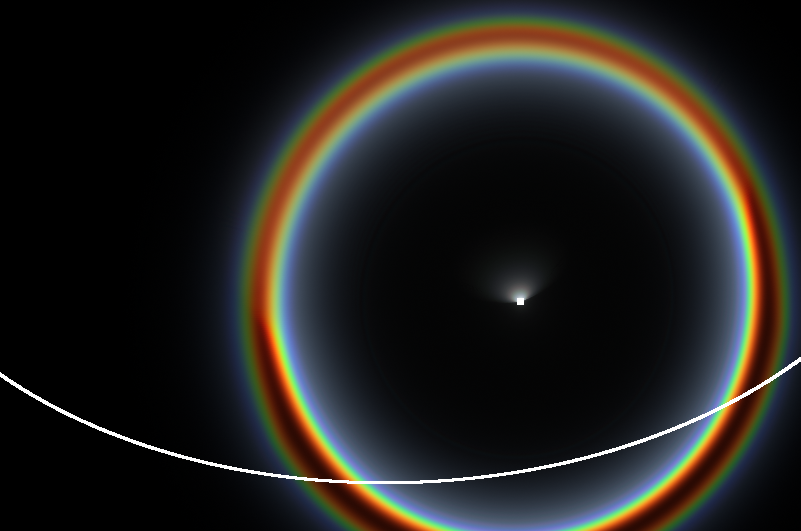
Anyway, on Aug 11^th, 2020, my instincts were right. Just before I finished work in Dresden-Langebrück, a moderate shower moved in from the northeast. The sunlight was somewhat dim, which resulted in an unspectacular primary rainbow from 17:15 CEST onwards. I could see some larger drops glint in the sunlight. I went to my car on the parking lot during the next minutes, and lost sight to the east, so I do not exactly know what happened later on this side of the sky. The rain was still ongoing, but not heavy, there were people cycling around without looking too much disturbed. I’m not entirely sure if it was still the same rain shower, or another one which had meanwhile moved in. I took three photos at the parking lot (17:23-24 CEST), and then drove about 100 m to a spot with a good view towards the west. There was nothing to be seen with the naked eye, just the sun, some glinting raindrops, a cloud, and blue sky below. A major problem is that raindrops will fall on the front lens, especially when using a fisheye objective that cannot be shielded and has to be held out of the car window to make proper use of its field of view. So one needs to be fast, otherwise the images will be spoiled by artifacts from the drops. That is why I did not do any image stacks, just a threefold exposure bracket per shot for safety (to have at least one picture with a useful exposure). In between, I had to wipe the lens dry. All of the ten shots I took there from 17:26-30 showed the tertiary rainbow after some processing, and it also appeared on the earlier pictures from the parking lot, as far as the view permitted. I was rather overwhelmed to see more than the complete upper half of the tertiary against the blue sky and cloud background when I first applied an unsharp mask to the images. The quaternary rainbow (located just outside the tertiary) can also be detected beyond any doubts, especially on the left side. I found no supernumerary arcs and no traces of the seventh order [4] (which I had missed to pay attention to during the observation, I also did not use any polarizers, and as mentioned, I did not record image stacks).

17:30:00 CEST, Pentax K-5, smc Pentax-DA fisheye 10-17 mm at f = 17 mm, f/14, 1/400 s at ISO 80, artifact-minimized processing by separate unsharp masking of color differences

Original image

Green minus blue color channel difference unsharp masked

Color differences unsharp masked

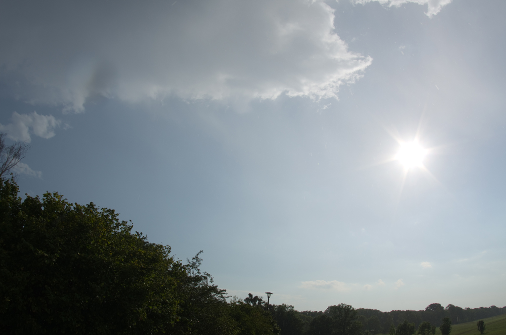
It is well known that aerodynamic flattening of larger raindrops has an impact on rainbows through the so-called Möbius shifts, but so far the consequences for higher order rainbows have only been studied theoretically. Are there any new insights from this observation? This, of course, requires an image calibration, i.e. the assignment of scattering coordinates (scattering angle and clock angle, i.e. the sun-centered azimuth, which I will count clockwise from the rainbow’s top here) to the individual pixels. The position of the sun is easily calculated from the time the respective photograph was taken (17:27:54 CEST for the top image, checked with a radio-controlled watch) and the location (51.13° N, 13.83° E), which gives in this case an elevation of 27.6° and an azimuth of 259.5°. The pixel coordinates of the sun’s center could also be reliably determined from an image version developed as dark as possible from the RAW file in Photoshop. The projection of this specific lens I had measured eight years ago (when I newly got it), but I did also a cross-check with recent starfield pictures (abundantly available from my attempts to catch Perseid meteors the following nights). In order to determine the relevant Euler angles (elevation and azimuth of the camera’s optical axis, and the rotation of the camera sensor chip around this axis), I still needed another reference mark. Luckily there was a telecommunication tower at the horizon which I could identify and then calculate under which elevation and azimuth it is seen from the observing location.

Technical sidenote: The two coordinates of the reference mark provide me indeed with one condition more than the number of available degrees of freedom, so I can check the overall consistency of the calibration. And here it initially turned out to be not very convincing. What went wrong? When checking my hidden assumptions I found that I had pinned the piercing point of the optical axis to the precise center of the CMOS sensor (in terms of pixel coordinates). This may not be realistic, and, moreover, in a Pentax K-5 camera the sensor can move several millimeters to compensate for shaking. Even with the shaking compensation turned off there is no guarantee that it will find and stay in the optical center position (plus, there are decentering errors of the lens). From the working principle of the calibration procedure I expect the decentering error to be of quadratic order, and it may turn out to be negligible for longer focal lengths. But it matters for a fisheye lens. So I used the amounts of decentering in X and Y as further degrees of freedom and achieved consistent results for a shift of 26 pixels (0.12 mm) in the horizontal (and zero in the vertical). However, a further reference mark would be needed for a truly unique determination. Then there would still remain the assumption of a rotationally symmetric lens, but this seems to be acceptable as indicated by the recent starfield test.

From an equilateral projection in scattering coordinates it can then be deduced that the tertiary does not bend significantly over the recorded range of clock angles, which also holds for the quaternary as far as it peaks out of the noise. So seemingly they appeared as perfectly concentric circles here!

Equilateral projection in scattering coordinates

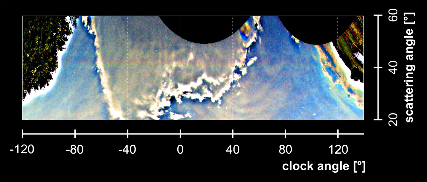
This is somewhat surprising, as theory predicts that these rainbows are also subject to Möbius shifts of various amounts along their circumference, which should become noticeable if larger (more distorted) drops are involved. Interestingly, for this sun elevation the Möbius shifts will move the tops of  the 3^rd and 4^th order rainbows towards each other. They might even overlap for an effective drop radius of 0.5 mm [5]. However, in nature, in most cases the drop size distribution (DSD) will cover a broad range of sizes, also including small drops. Because the shape distortion sets in (at least) quadratically with rising drop radius, it is likely to see some of the traditional concentric sphere-drop rainbows shine through in the full mixture of size dependent rainbows. This I already noted in simulations using broad Marshall-Palmer DSDs (i.e. a simple decaying exponential). As mentioned, there was no heavy rainfall going on during the observation on Aug 11^th, so a dominance of the less distorted smaller sizes can be reasonably assumed – regrettably there are no direct measurements of the DSD. Lee and Laven [1] argue that broad DSDs tend to wipe out the tertiary’s top and leave only the sides, but their analysis was based on much lower sun elevations than occurring here.

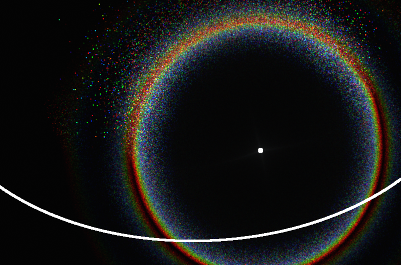
So in order to see how much the concentricity of the tertiary and quaternary rainbows will be affected in this specific case I did some simulations for the proper sun elevation and a (guessed) DSD which contains mostly small and moderate sized drops: A Marshall-Palmer with decaying parameter (Lambda) of 4 mm^-1, as previously used [5]. There are two complementary simulation methods which I can apply: 1) GO: Geometric optic raytracing (including polarization, but neglecting interference and diffraction) for all rainbow orders up to the 7^th, based on a Beard-Chuang cosine series drop shape model, with optional (2,0) quadrupole mode oscillations and Gaussian tilts of the symmetry axis from the vertical, and 2) DMK: Debye series calculations for spherical drops of various sizes, superimposed in intensity after being shifted in scattering angle by the appropriate Möbius value (depending on drop size, rainbow order, and clock angle, following Können [6]). These calculation include only rainbow orders up to the 5^th. The Möbius shifts themselves are taken from a look-up table comprising earlier raytracing results. These were calculated from a simpler shape model (two conjoined half spheroids fitted to Beard-Chuang shapes) and do not include drop oscillations or tilts for the higher-order rainbows yet. However, this second method has the advantage of showing if supernumerary arcs can be expected under the given conditions.

I removed the most disturbing directly transmitted light (sometimes referred to as “zero order glow”) as well as the less important contributions from external reflection and the lowest two rainbow orders from the simulation, and show the resulting clear higher-order rainbows in the same sunward projection (and for the same sun elevation) as in the top image. As a reference, I also let simulations run for spherical drops with the same DSD. These, of course, turn out perfectly concentric (in scattering coordinates, not necessarily in the projected image). After having switched on drop distortions, it is reassuring to see that both methods agree in keeping the upper halves of the tertiary and quaternary well separated and still nearly concentric. However, a tendency to blur these parts can be noted, due to the contribution of larger drops. Two more pieces of information can be extracted here: Introducing moderate axis tilts and (2,0) oscillations (both their amplitude distributions set to the “standard values” used in [7]) does not lead to visible changes in the result (GO), and supernumeraries do not appear, neither for flattened nor spherical drops (DMK).

GO sphere reference simulation

GO distorted drops, no oscillations, no tilts

GO distorted drops, with oscillations and tilts

DMK sphere reference simulation

DMK distorted drops, no oscillations, no tilts

The latter result illustrates that in broad DSDs supernumeraries need the stabilizing “Fraser mechanism” [8] to become visible: If, with increasing drop size, the Möbius shifts grow in the opposite direction than the supernumeraries’ convergence towards the Descartes angle due to their shrinking angular width, there will be a certain critical drop size at which these effects compensate. Because of the resulting position stability against changes of drop radii, the supernumeraries of drops around the critical size will peak out from the unstructured background of superimposed non-aligned supernumeraries of other sizes. Traditionally, this argument is invoked for the primary rainbow (with a critical drop radius of about 0.25 mm for the first supernumerary), but it holds likewise for all other orders [9]. If the Möbius shifts have the wrong sign (as for the tertiary and quaternary bows at the sun elevation of my observation) or are set to zero (as in the sphere reference simulations), there exists no compensation point and the averaging of all supernumeraries results in a more or less uniform intensity gradient.

The GO simulations reproduce also the 7^th order rainbow, but, under the assumed conditions, do not predict any amplification effects for it caused by drop distortions or oscillations. In fact, it is not even recognizable in the simulation pictures shown here, but can be extracted by a larger intensity-to-RGB-value scaling factor (or higher gamma value).

In conclusion, the observed concentric tertiary and quaternary rainbows without supernumeraries can be consistently interpreted in the current theoretical framework of broad raindrop size distributions and drop shapes with aerodynamically plausible amounts of flattening and oscillations. Even though shape distortions have a larger influence on higher orders, they do not forbid that traditionally shaped rainbows are formed, if enough small drops are present. Of course, any observations of genuine non-spherical drop effects such as higher order twinned bows are highly welcome as they would allow for a more challenging test of the simulation models.

A multi-split rainbow from south-east China, August 12th, 2014

 

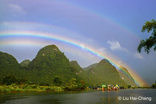
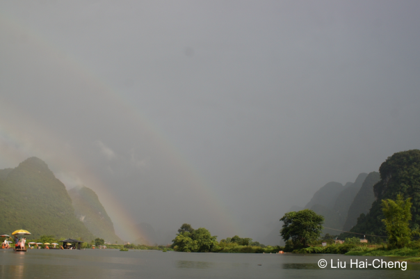
Yulong river, Guangxi province, August 12^th, 2014, 17:18 Chinese standard time

Twinned rainbows are rare sightings, in the sense that one may see on average only one per year in Central Europe even when paying close attention. Much rarer still, and maybe restricted to regions closer to the equator, are multi-split rainbows. Only few cases have been documented so far [1, 2, 3], though more snapshots can be found on image sharing platforms labeled as “triple rainbow” etc. It is always a very favorable situation if an archivist and analyst like myself can establish direct communication with a skilful observer, who recorded details of a rainbow display that provide some insight beyond the pretty pictures.

In April 2019 I emailed Mr. Ji Yun, who manages a Facebook group dedicated to atmospheric optical phenomena in China, asking about a spectacular photograph of a multi-split rainbow which had been shared there. He kindly relayed my request to Mr. Liu Hai-Cheng, the original observer. Mr. Liu agreed to answer a long list of questions and I also received two sets of photographs from August 12^th, 2014, one from his Sony NEX-5C camera (equipped with a Nikon AF 28mm f/2.8 lens) and the other from his cell phone (Coolpad 8720L). The camera clock’s time stamps were calibrated with respect to the actual local time by comparing camera and cell phone pictures, and assuming the cell phone clock to be synchronized over the network. All time data are given here in Chinese standard time (UTC+8h).

Mr. Liu observed this rainbow rarity in the beautiful landscape of the karst mountains near the Yulong bridge (Yangshuo County, Guilin City, Guangxi province, about 400 km northwest of Hong Kong, 24.8° N, 110.4° E) during a boat trip on the Yulong river. He remembers that it was very hot that afternoon. It began to rain before he passed through the tunnel of the bridge (at about 16:50), with some heavier rain lasting for about 25 minutes. There was no lightning, thunder or strong wind.

Judging from the photos, the rainbow appeared at about 17:10 within 30 s or less. Already on the early photographs there are hints of the unusual splitting of the primary:

17:11

However, Mr. Liu’s visual impression was that the splitting became prominent only later, after the (seemingly ordinary) primary and secondary bow had appeared successively. He also noted that the visibility of the split branches changed over time, while the main primary could always be seen clearly.

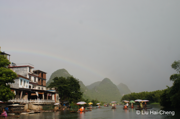
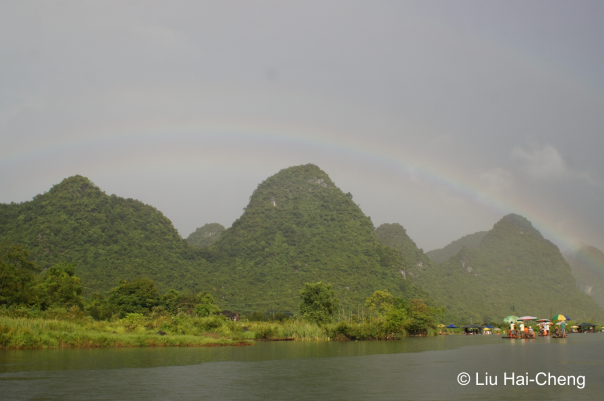
Towards the end of the shower, the display reached its peak quality. The following pictures cover the full right-hand side of the rainbow and some of the left. They are presented without additional filtering to allow for a better assessment of the natural contrast conditions.

17:18 (unfiltered version of the title image)

17:18

17:19

For a deeper analysis, I chose the title picture, recorded at 17:18. In the contrast-enhanced version, three primary branches are directly visible, with the most intense one in the center. The secondary rainbow, as far as it is included in the frame, does not exhibit any anomalies. This is a typical feature in (almost) all split rainbow observations known so far. My goal was now to transform the photograph into the scattering angle vs. clock angle coordinate system (in equirectangular projection), as I did on previous occasions [1, 4]. The scattering angle is the angular distance from the sun, and the clock angle the azimuth around the rainbow’s circumference, with the 0° position corresponding to its top.

The sun’s position is easily obtained from standard astronomy software (giving an elevation of 25.4°, and azimuth of 275.4°). Additionally, the precise focal length of the lens (in pixel units) and distortion characteristics need to be known, as well as the camera pointing direction in elevation and azimuth, and the angle describing the rotation of the sensor’s pixel grid with respect to the vertical.

To precisely determine these quantities, a rather extensive calibration must be carried out. Here I had to try some reasonable guessing: There is a nominal focal length in mm, the sensor data (pixel pitch) can be looked up, as well as some distortion information for this specific lens. From aerial pictures showing the river and individual mountains, the viewing direction can be estimated. The appearance of the water surface gives some clues about the camera rotation. In combination, all these estimations allow for a plausible transformation:

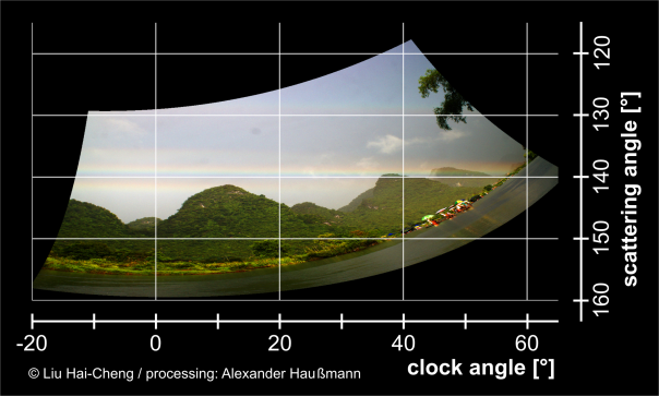
Assuming this reconstruction to be not too far off, it is immediately obvious that the bright central branch does indeed fit to the conventional primary rainbow locus at a constant scattering angle of about 138°. As expected, the secondary ends up at about 129°, also as a straight line. The lower branch (i.e. at higher scattering angles) can in principle be explained by aerodynamically flattened raindrops, following a long tradition in rainbow physics [5, 6, 7, 8, 4]. However, the upper branch penetrating into Alexander’s dark band requires elongated raindrops, whose existence cannot be accounted for by aerodynamics alone. Electrostatic fields [9] can elongate raindrops, but in the absence of any lightning activity it is speculative if any higher fields were present. Elongated shapes do also occur as transitory states during oscillations of larger drops in the appropriate (axisymmetric) modes [10].

The problematic element in this explanation is, however, that in the case of the rainbow we deal with a large number of contributing raindrops and a temporal average due to the finite exposure time. So we need an argument why contributions from transitory states are not simply wiped out. The resonance frequencies of the individual drops depend on their size, so no singular event such as an acoustic shock wave from thunder (if there had been any at all) can synchronize the oscillations. The only plausible idea for a formation of stable rainbow branches by drop oscillations in a stochastic ensemble might be that the two extremal states of the oscillation (flattened and elongated) are encountered with a higher probability than intermediate ones, as the momentary velocity decreases to zero at the turning points of any classical oscillation. Admittedly, this requires a rather narrow distribution of amplitudes throughout the ensemble (at least in the dominant drop size range), as otherwise the branches will be wiped out again due to the spread in extremal axis ratios. To my knowledge, there is not enough data on the statistical properties of oscillations in large ensembles of natural raindrops published yet to draw a definitive conclusion here.

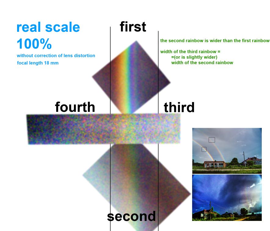
Some further details of this observation are worth to be noted: The three branches of the primary bow appear each in a distinct fashion: The lowest is broad and rather diffuse, the middle one is bright and shows the features of a typical primary rainbow, the top one is narrow with a sharp uppermost outer rim. Moreover, it gives the impression of having developed a downward sub-branch in the –10°…+5° clock angle interval, resulting in a four-fold split bow there.

Rainbows certainly go on fascinating people all over the world, and rightfully so: Even in the 21^st century, some outstanding displays occur from time to time that still challenge our understanding. Maybe those in hotter climates with intense rain showers have better chances of catching such rarities. In any case, we have to go out and take a look and a picture at the right time.

Glories and cloudbows observed during short-distance flights

On Sept 25^th and 27^th, 2014, I was traveling by plane from Dresden to Brussels and back, with stops at Frankfurt and Munich, respectively. As usual, I booked window seats to study sky phenomena. The sunward side was not very interesting, since these short-distance flights are carried out at heights below the cirrus clouds and therefore no sub-horizon halos can be observed (at least in autumn). On Sept 25^th only a single 22° halo appeared in the cirrus clouds above the plane, whereas on Sept 27^th ice crystal clouds seemed to be fully absent.

Accordingly, the viewing direction towards the antisolar point proved to be much more interesting. As most of the Atmospheric Optics enthusiasts I had seen glories and cloudbows before (especially when traveling to the Light&Color meetings in the US) but this time the conditions seemed to be especially favorable. I could observe an an almost textbook-like development of both phenomena right after piercing through an Altocumulus layer after the take off from Dresden (Sept 25^th, 11:13 CEST):

From Debye series simulations (intensity sum of the p = 0 to p = 11 terms in order to prevent artifacts from the small-scale inter-p-interferences as present in the Mie results) a mean drop radius of about 8 µm with 0.5 µm standard deviation can be estimated (assuming a Gaussian drop size distribution):

This simulation was calculated for the original lens projection with added ad-hoc gray background. It is also available as a fisheye view centered on the antisolar point without background [1], together with the corresponding simulation for monodisperse drops (no spread in size) of 8 µm in radius [2].

Unsharp masking and saturation increase processing of the photograph reveals that the sequence of supernumeraries can be traced until they merge with the glory rings:

Over the next minute I mounted the fisheye lens to my camera in order to record a broader view. Unfortunately, some of the outer glory rings and inner supernumeraries had already vanished, indicating an increase in the drop size spread:

Note the smaller angular size of the plane’s shadow as the distance to the Ac layer had further increased. A well fitting simulation to this photo can be calculated by assuming again a mean drop radius of 8 µm and setting the standard deviation now to 1 µm:

For comparison, the fisheye simulation centered on the antisolar point was calculated for the 1 µm drop size spread as well [3]. Furthermore, I recorded a video sequence showing the movement of both glory and cloudbow across the uniform Ac layer (11:15, [4]). When later the edge of the Ac field was reached, the glory showed an appreciable degree of distortion (11:18 CEST [5], processed version [6]).

On Sept 27^th, not a uniform but a fractured Ac layer was present after the take off from Brussels. Nonetheless the glory appeared circular (12:34 CEST [7], processed version [8], video at 12:37 CEST [9]), with the exception of occasional larger disturbances in the layer (12:34 CEST [10]). The cloudbow was not as prominent as two days earlier. During the later part of the flight only occasional Cumulus clouds were present, which did not allow for further glory observations until the plane started descending when approaching Munich. At this point the angular size of the clouds became large enough again to act as suitable canvas for the glory (13:14 CEST [11] [12]). During the final passage through a Cu cloud I recorded a further video (13:15 CEST [13]). Remarkably, the angular size of the plane’s shadow varies rapidly (indicating the distance to the drops) whereas the the angular size of the glory remains rather stable (indicating the drop radius).

Photos and videos were taken with a Pentax K-5 camera equipped with either a Pentax 10-17 mm fisheye or Pentax-DA 18-55 mm standard zoom lens. A gallery view of my photos can be seen here [14].

Alexander Haußmann

Fraunhofer lines in rainbow ?

Fraunhofer lines are dark lines in the sun’s spectrum. They are caused by resonant atomic absorption of the sun’s thermal continuum radiation by photospheric gases.

The lines provide clues to the chemical composition of the solar atmosphere, as well as its physical conditions like temperature, pressure, magnetic fields etc.

My rainbow photography dated 11.Oct.2013 showed some greyish bands in the yellow.

Are they traces of the strongest Fraunhofer lines or artifacts of the camera’s sensor being unable to profile intermediate colors?
Is it possible at all to obtain spectral lines in nature without a prism or grating?

Author: Michael Großmann, Kämpfelbach, Germany

Neklid Antisolar arcs: Case closed?

In my last post I outlined several possibilities to explain the great brightness of the antisolar arc (AA) compared to the heliac arc (HA) in the Neklid display from Jan 30^th, 2014. All of them were a bit off the main road of traditional halo science, but traditional arguments did not help to clarify what was observed, hence I had to look for something else.

Both the concepts of plate Parry crystals and trigonal Parry columns should yield weak traces of unrealistic (or better to say non-traditional) halos that might appear in a deeper photo analysis. Claudia Hinz provided me with a set of pictures from the display to unleash any kind of filters that would seem appropriate. Indeed it was possible to pin down traces of the Kern arc in some of the pictures after the initial application of an unsharp mask (1, 2), followed by high-pass filtering (1, 2) or, alternatively, by Blue-Red subtraction (1, 2). Note that the Kern arc was weakly present in the simulations for hexagonal, Parry-oriented plates. This, of course, must not be confused with the recently proven Kern arc explanation relying on trigonal plates in plate orientation. Finally, trigonal columns in Parry orientation are a third non-traditional crystal configuration giving rise to new halos. However, these do not yield a Kern arc.

Obviously, the Kern arc fragments in the photos are very feeble and the whole procedure reminds a bit of the search for higher order rainbows. It is mere guesswork to detect how far the arc stretches around the zenith, but doubtlessly it extends up to 90° and more in azimuth, thus being clearly distinguishable form the circumzenith arc. Nonetheless, one would feel safer with further evidence. Comparing the simulations for Parry columns and Parry plates, three more differences are discernible (apart from the changed AA/HA ratio):

1) For Parry plates, the upper suncave Parry arc does not show an uniform brightness, but appears brighter directly above the sun and loses some intensity towards the points where it joins the upper tangent arc.

2) The upper loop of the Tricker anthelic arc is suppressed for columns, but shows up for plates.

3) Some extensions of the upper Tape arcs appear between the Wegener arc and the subhelic arc.

At least the first two points can be answered in favor of the Parry plates, being visible even without strong filtering. However, I failed to detect any extended Tape arcs as “ultimate proof” so far. This might not surprise since they are, according to the simulation, comparable to the Kern arc in intensity and appear in regions of the sky where the crystal homogeneity was not as well developed as in the vicinity of the zenith.

Piecing the parts together, it seems evident that at Neklid the AA intensity was due to Parry-oriented hexagonal plates. Their traces were detectable, whereas nothing appeared that would hint on trigonal Parry columns. In contrast to this, Parry trigonals were responsible in Rovaniemi 2008. This implies that in nature at least two different mechanisms occur for AA brightening.

Finally the question remains how plates may get into a Parry falling mode. But as long as no one understands how symmetric columns do this (though we have the empirical evidence), we should be prepared for surprises. There might also be a connection to recently discussed details of the Lowitz orientation (2013 Light and Color in Nature conference, talk 5.1).

The mystery of bright antisolar arcs

 

 

(photo by Claudia Hinz)

The antisolar (or subanthelic) arc (AA) was one out of the vast range of halo species occurring during the marvelous Neklid display observed by Claudia and Wolfgang Hinz on Jan 30^th, 2014. This kind of halo seems to be exceedingly rare, since it has only been documented during the very best displays, mostly observed in Antarctica. On the other hand, the heliac arc (HA) is a, however not frequent, but well-known guest in Central Europe. Both of them are reflection halos generated by Parry oriented crystals and touch each other at the vertices of their large loops. Fisheye photos towards the zenith from Neklid shows both these halos in perfect symmetry and approximately similar intensity, at least regarding the upper part of the AA.

When trying to simulate the display (solar elevation 17.5°) using HaloPoint2.0, I noticed that the AA was rendered much weaker than the HA, which of course does not match the photographic data. To obtain the Parry effects (Parry arcs, Tape arcs, HA, AA, Hastings arc, partially circumzenith arc, Tricker arc, subhelic arc) I chose a population of “normal” (i.e. symmetrically hexagonal) column crystals with a length/width ratio of c/a = 2 in the appropriate orientation. Since both HA and AA are generated by this very same crystal population, their mutual intensity ratio cannot be influenced by adding plates, singly ordered columns, or randomly oriented crystals. This mysterious issue has also been noted by a Japanese programmer who came across the Neklid pictures.

Inclusions of air or solid particles within the ice crystals are an obvious hypothesis to explain this dissenting AA/HA intensity ratio, since they cannot be accounted for in the standard simulation software. However, a look into literature reveals that there are external and internal ray paths for the HA, but only internal paths for the AA ([1] p. 34-35). That means that inclusions will diminish the AA to a greater extent than the HA. In the extreme case with the interior totally blocked, no AA can arise but a HA is still possible due to external reflection at a sloping crystal face. Hence inclusions cannot explain the bright AA from the Neklid display. Air cavities at the ends of columns which are seen quite often in crystal samples will also inhibit the AA because an internal reflection at a well defined end face is needed for its formation.

Spatial inhomogeneities in the crystal distribution might serve as explanation as long as there is only one single photo or display to deal with, especially when the air flow conditions are as special as they were at Neklid. Maybe there were just “more“ good crystals in the direction of the AA compared to where the HA is formed, either by chance or systematically due to the wind regime. But surprisingly also the observations from the South Pole (Jan 21^st, 1986 (Walter Tape); Jan 11^th, 1999 (Marko Riikonen), also discussed here) show an AA/HA ratio somewhere in the region of unity as far as one can guess from the printed reproductions ([1] p. 30, [2] p. 58). Parts of the AA appeared even brighter than the HA in Finnish spotlight displays. All this implies a deeper reason for the AA brightening. It seems rather unlikely that in all these cases the inhomogeneities should have worked only in favor of the AA.

Hence the crystals themselves must be responsible for AA brightening. Non-standard crystal shapes and orientations are conjectures that can be tested easily with the available simulation programs. For a first try, one can assign a Parry orientation to plates instead of columns. Changing the c/a shape ratio from 2 to 0.5 while keeping all other parameters fixed results in a much brighter AA.

It is, however, commonly accepted that due to the air drag only columns can acquire a Parry orientation ([1] p. 42). Furthermore, some halos appear in the plate-Parry simulation which have not been observed in reality, e.g. a weak Kern arc complementing the circumzenith arc. At this stage the question may arise why only due to aerodynamics any symmetric hexagonal crystal (may it even be a column) should be able to place a pair of its side faces horizontally to generate Parry halos such as the HA and AA. Cross-like clusters or tabular crystals ([1] p. 42), from whose shapes one will immediately infer that rotations around the long axis are suppressed, seem much more plausible. Surprisingly, Walter Tape’s analysis of collected crystal samples shows that Parry halos are mainly caused by ordinary, symmetric columns. Parry orientations might be a natural mode of falling for small ice crystals, though up to now the aerodynamic reasons remain unclear. Nonetheless I tested if tabular crystals would give a bright AA. This was neither the case for moderate (height/width = 0.5) nor strong aspect ratio (height/width = 0.3). The AA was in both cases even weaker than in the symmetric standard simulation with which the discussion started.

Trigonal plates have been brought into discussion as possible crystal shapes being responsible for the Kern arc (see also [1] p. 102). Out of curiosity I tested how Parry oriented trigonal columns would affect the AA/HA intensity ratio. In contrast to symmetric hexagonal columns two different cases exist here, depending on whether the top or bottom face is oriented horizontally. As seen from the results, a sufficiently bright AA can be simulated using trigonal Parry columns with horizontal bottom faces, but the upper suncave Parry arc and the lower lateral Tape arcs at the horizon disappear. Obviously they have to, since a trigonal crystal in this orientation does not provide the necessary faces for their formation. On the other hand, the simulation predicts unrealistic arcs like the loop within the circumzenith arc. Choosing a trigonal Parry population with top faces horizontal will diminish the loop of the HA and wipe out the upper part of the AA as well as the upper lateral Tape arcs and add an unrealistic halo that sweeps away from the supralateral arc.

Is it possible to generate a realistic simulation of the Neklid picture with such crystals? Clearly this will require to add a second Parry population of symmetric hexagonal prisms. Doing so, a reasonable compromise can be achieved. In this case the hexagonal crystals produce the Parry arc, whereas the trigonal ones are responsible for the AA. Due to the triangular portion being small, the unrealistic halos become insignificant. However, the fact that a further degree of freedom (mixing ratio trigonal/hexagonal) has to be added to the set of initial simulation parameters is somehow dissatisfying.

The question lies at hand if this result might also be obtained by choosing a single Parry population of intermediate shapes between the symmetric hexagonal and trigonal extremes. This idea is further motivated through pictures of sampled crystals that, though being labeled „trigonal“, show in fact non-symmetric hexagonal shapes. The simulation for these shapes does indeed predict an enhanced AA compared to symmetric hexagons, but the lower lateral Tape arcs and the upper suncave Parry arc still appear too weak. This means that an additional set of symmetric hexagonal crystals is needed again to render these halos at the proper intensity.

Moreover, quite prominent unrealistic halos like the loop crossing the circumzenith arc appear in the simulation. If this assumption for the Parry crystal shape was right, this arc should be visible in an unsharp mask processing of the photos. Its absence hints that these crystals did not play a dominant role in the Neklid display. One could argue that the unrealistic halos may depend strongly on the actual crystal shape and might be washed out in a natural mixture of different “trigonalities“. However, the simulation tests indicate that even in this case the unrealistic halos remain rather strong, as long as one still wishes to maintain an AA at sufficient intensity.

As a conclusion, it can be stated that the intensity ratio between the heliac arc and the antisolar arc in the Neklid display as well as in Antarctic and Finnish observations has raised basic questions about the shapes of the responsible crystals. Simulations with symmetric hexagonal Parry columns, i.e. the standard shapes, render the AA to weak compared to the HA. Inclusions in the crystals and spatial inhomogeneities of the crystal distribution can be ruled out as the cause of this deviation. Plates in Parry orientation or a mixture of Parry oriented trigonal columns with horizontal bottom faces and hexagonal columns both result in a more realistic AA/HA intensity ratio. However, they introduce traces of unrealistic halos and are rather uncommon hypotheses: Plate crystals are not supposed to fall like this, and the existence of “true” trigonal crystals is doubtful. Moreover, the trigonal crystals need an accompanying set of standard Parry crystals to generate other halos like the upper suncave Parry arc.

So all in all the mystery of bright antisolar arcs cannot be regarded as solved at this stage. Since this halo species is very rare in free nature, it might be helpful to test perspex crystal models of different shapes in Michael Großmann’s “Halomator“ laboratory setup. Though the refractive index in perspex is higher than in ice, the basic relations between HA and AA stay the same. However the big challenge remains to collect and document crystals during such a display, e.g. with the methods described by Reinhard Nitze.

References

[1]     W. Tape, Atmospheric Halos (American Geophysical Union, 1994)

[2]     W. Tape, J. Moilanen, Atmospheric Halos and the Search for Angle x (American Geophysical Union, 2006)

Addendum

I missed an important piece of information from Finland 2008: The idea of trigonal crystals making Parry halos was already pointed out by Marko Riikonen in an analysis of the Rovaniemi searchlight display. In that case, even one of the halos that I termed “unrealistic“ was observed in reality, thus strongly supporting the trigonal interpretation.

3rd and 4th order rainbows – technical details

The lens has a distortion, but nevertheless I tried to compare the width of the first, second and third order rainbows. I selected three fragments, each of them at an approximately identical distance from the center of the photo to get an identical distortion.

The first order rainbow has supernumeraries.

The second order rainbow seems to be wider than that of the first order.

The width of the third order rainbow appears the same as or greater than that of the second order rainbow. The digital colour noise didn´t allow an exact comparison.

I tried to calculate the width of the rainbow, it seems to be between 1 and 5 degrees, but I think it is probably 2 or 3 degrees (graphic 1 and 2).

 

I estimate the radius of the third order rainbow at about 39 to 43 degrees, with the blue colour at 39 and the red colour at 43 degrees. It seems to me that the brightest part of the rainbow had a radius of 41 degrees, but it also was very faint. I don´t know which colour corresponds to this radius, I think it is green or perhaps yellow. It is difficult to see because of the colour noise.

Author: Sergei Antipov, Russia

Light refraction in a sunshine recorder

Only at very rare occasions, light refraction can be seen as impressive as in this example. The photo was taken by Hermann Scheer at the Meteorological Observatory on Mt. Hoher Sonnblick (3105m) in the Hohe Tauern mountains in Austria. A layer of ice and rime had formed on the glass sphere of the Campbell Stokes sunshine recorder. This layer split the sunlight up into its spectral colours. That is how impressive physics can be.

Reconstruction of height and position of the green airglow from July 15th, 2012

It was an ironic situation when during the night from 14^th to 15^th of July 2012 (at a weekend) a high number of observers and photographers were looking for a predicted aurora borealis and instead were confronted with a remarkable outburst of structured (or banded) green airglow. This phenomenon is well known and explored by professional geo-scientists but seemed to have slipped the attention of most amateur observers, including myself, up to then. Though it first seemed likely that the geomagnetic storm may have somehow triggered this event, later observations (e.g. July 23^rd, 2012: http://www.polarlichter.info/airglow.htm) indicated that the traditional excitation mechanism (UV and X-Ray radiation from the sun) is capable of producing intense green airglow without the need for a geomagnetic anomaly.

Due to the fascination I felt during my own observation, I got interested in using the many available photographs from the July 14^th/15^th night for a height and position reconstruction. However, as I later found out from literature, the airglow height of  87-95 km (i.e. a quite thin layer, comparable to the NLC layer around 83 km) is already well established by professional measurements. It is remarkable that this value can in fact be reproduced by comparing amateur photographs from various locations in Germany by an un-biased analysis, which I want to present here.

The first task to do was to contact other observes via the well-known communication boards about atmospheric optics to gather suitable photographic material. Of course I had my own images at hand and intended to use them for this process, so I already had a list of time slots to find synchronous counterparts for. Even though I could find several pictures taken within a tolerance of < 1 minute with respect to my own photos, I had to drop most of them since a coarse analysis of the viewing directions yielded no overlapping fields of view. But through discussing my idea with several other photographers, I was able to identify other matching pairs independent from my own material. Finally, I ended up with two data sets (image pairs), 1 and 2,  to work with:

1a) Frank and Sabine Wächter: July 15^th, 00:55 CEST, 51° 12’ N, 13° 35’ E, 189 m above sea level (Meißen, Saxonia): https://dl.dropbox.com/u/8849406/Forum/AirglowBlog/1a.jpg

1b) Jens Hackmann: July 15^th, 00:55 CEST, 49° 29’ N, 9° 55’ E, 333 m above sea level (Weikersheim, Baden-Württemberg): https://dl.dropbox.com/u/8849406/Forum/AirglowBlog/1b.jpg

2a) Franz Peter Pauzenberger: July 15^th, 02:02 CEST, 49° 00’ N, 11° 30’ E, 518 m above sea level (Beilngries, Bavaria): https://dl.dropbox.com/u/8849406/Forum/AirglowBlog/2a.jpg

2b) Alexander Haußmann: July 15^th, 02:01 CEST, 51° 32’ N, 13° 58’ E, 110 m above sea level (Senftenberg, Brandenburg): https://dl.dropbox.com/u/8849406/Forum/AirglowBlog/2b.jpg

For a detailed analysis, it is necessary to calibrate these photos, which means to precisely assign values for azimuth and elevation to each pixel. If the projection characteristics of the photographic lens are known, the positions of two stars in each picture are sufficient input for this purpose. However, the simple assumption of an ideal gnomonic (rectilinear) or equal-area projection (for ordinary and fisheye lenses, respectively) drastically limits the accuracy of the results. To overcome this, the projection characteristics for all four lenses were reconstructed by measuring the pixel distances of approximately 15 stars from the image center and compare these with the angular distance from the optical axis for each image.

After this calibration and assignment, longitude and latitude positions for each pixel can be calculated, allowing the projection of the photo onto a map if a certain height of the airglow layer is assumed. This method already proved to be very useful for the reconstruction of NLC positions (http://www.meteoros.de/php/viewtopic.php?t=8451). Since the goal is here to determine the layer height, this parameter is varied until the corresponding structures in both reconstructions of an image pair give the best fit. Indeed it was possible to find consistent height values for both data sets, 92 km for pair 1 (https://dl.dropbox.com/u/8849406/Forum/AirglowBlog/1.gif) and 93 km for pair 2 (https://dl.dropbox.com/u/8849406/Forum/AirglowBlog/2.gif). Here the traditional blink comparison technique was applied in a modern form using gif animations. It is fascinating to see how the airglow structures that look completely different in the original two photos of each pair coincide in the reconstruction on the map. Evidently, all non-airglow structures such as trees, background light, clouds, photographic violet aurora etc. have to be ignored in the reconstruction. It should be noted that more complex approaches (http://www.opticsinfobase.org/ao/abstract.cfm?uri=ao-51-7-963) are recently established in the professional field, allowing even to resolve finer structures within the thickness of the airglow layer.

Furthermore, these reconstructions show an undistorted view on the band structure of the green airglow layer. As already expected from the perspective view of the original photos, these bands are roughly aligned in the direction from West to East. Using the consistent height information obtained from the image pair comparisons, it is moreover justified to project a whole picture series from a single observation site onto the map in order gain insight in the airglow band dynamics. For this purpose I used a time lapse series that I took from July 14^th, 23.16 CEST to July 15^th,  01.20 MESZ at the Senftenberger See (51° 29’ N, 14° 01’ E), starting in the evening dawn and originally intended to capture the predicted aurora borealis (https://dl.dropbox.com/u/8849406/Forum/AirglowBlog/3.avi). Due to the weak contrast of the airglow at this stage, strong image processing is needed to separate the bands from the background. Though this finally results in a rather poor signal to noise ratio, it can clearly be seen that the airglow bands move in northward direction (https://dl.dropbox.com/u/8849406/Forum/AirglowBlog/4.avi), illustrating the recombination and/or matter transport dynamics in the mesopause region.

Author: Alexander Haussmann

Polarized Light in Nature

My book “Polarized Light in Nature” is now online available.

The pdf can be downloaded from my site, www.guntherkonnen.com. Go to English/Articles and scroll down to the year of publication (1985). The size of the download is 24 Mb.

The Dutch version (1980) can also been downloaded from the site (18 Mb).

Direct access is also possible:
http://s3.amazonaws.com/gunther-konnen/documents/249/1985_Pol_Light_in_Nature_book.pdf?1317929665 (English version)
or
http://s3.amazonaws.com/gunther-konnen/documents/246/1980_Gepolariseerd_Licht_boek.pdf?1317928523 (Dutch version),
but these addresses may change in case my site migrates to another server.

Author: Günther Können, Netherlands